Super Basic SDFs

In a recent experimental 2D gamedev project, I wanted to play around with drawing a bunch of game entities purely algorithmically rather than creating sprites for each of them. One important technique I ended up using was Signed Distance Fields (SDFs). In this post, I’ll go over the most basic implementation (we’ll draw a circle!) and explain how and why it works.

I should mention, before starting, that using SDFs for each of those entities was a bad idea since they have to be calculated for each frame, which is can be much more expensive than pre-rendering a bunch of animations stored in textures. Still, there are legitimate applications for this technique, such as in Valve’s famous 2007 font rendering white paper or for only a few elements. The main benefit is that the animation frame generation is continuous and limited only to the processing speed of the GPU rather than limited by however many frames your sprite animation contains. Yet, you can imagine how this is a double-edged sword as draw complexity increases.

How Does It Work?

An SDF function returns the distance from a given point to the limit of a particular shape. The simplest demonstration would be the SDF of a circle:

function sdf(vec2 pos, float radius) {
  return length(pos) - radius;
}

This function returns the distance from point pos to the origin (0,0) minus some arbitrary radius, meaning that any value that falls inside of that radius is negative while any number outside of it is positive.

In Practice

Let’s create a simple fragment shader to visualize this:

#version 330
in vec2 fragTexCoord;

out vec4 finalColor;

float sdf(vec2 pos, float r) {
    return length(pos) - r;
}

void main() {
    // center the coordinate system
    vec2 uv = -fragTexCoord.xy * 2.0 + 1.0;
    // calculate the sdf for the current fragment
    float d = sdf(uv, 0.5);
    finalColor = vec4(vec3(d), 1.0);
}

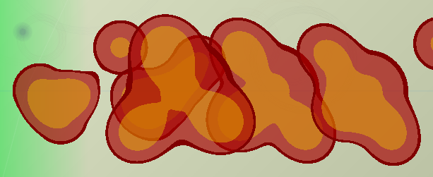
Rendered, centering the origin on the screen, with a width and height of 1, and applied to each pixel, it looks something like this:

You can see a pure black circle at the center of the image (negative values), with gray extending out the extremes of the image (positive values). Notice also how the corners are brighter as they are further away from the center.

Crisp Edges

Great for visualization, but a fuzzy circle isn’t too useful in practice. In order to truly visualize just a circle, we can apply the GLSL step function to normalize the value.

genType step(float edge, genType x);
For element i of the return value, 0.0 is returned if x[i] < edge[i], and 1.0 is returned otherwise.

This means that any value inside the circle will be black and any value outside of the circle will be white if we apply the output on the RGB channels of the output color:

void main() {
    // center the coordinate system
    vec2 uv = -fragTexCoord.xy * 2.0 + 1.0;
    // calculate the sdf for the current fragment
    float d = sdf(uv, 0.5);
    // normalize the output
    d = step(0.0, d);
    finalColor = vec4(vec3(d), 1.0);
}

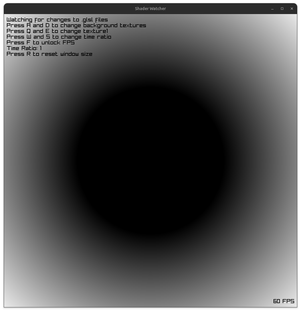
The output:

Much better. The circle is now clearly drawn onto the screen, with a very crisp boundary delimiting what’s inside and outside the radius.

Too Crisp?

Of course, this is a bit too crisp. In most contexts, everything drawn onto the screen is smooth and anti-aliased, so having a single standout like this looks awkward. We can soften the transition between the boundaries using the GLSL smoothstep function.

genType smoothstep(genType edge0, genType edge1, genType x);
smoothstep performs smooth Hermite interpolation between 0 and 1 when edge0 < x < edge1. This is useful in cases where a threshold function with a smooth transition is desired.

Replacing the step function with smoothstep:

void main() {
    // center the coordinate system
    vec2 uv = -fragTexCoord.xy * 2.0 + 1.0;
    // calculate the sdf for the current fragment
    float d = sdf(uv, 0.5);
    // normalize the output, but smoooothly
    d = smoothstep(0.0, 0.01, d);
    finalColor = vec4(vec3(d), 1.0);
}

It looks much smoother, but depending on your tastes, the edges might looks a bit too smooth, borderline blurry. This is where the limits of the demonstration begin to show. In a “real” setting, you wouldn’t hardcode the edge limits, but likely drive it relative to some other value, likely viewport scale or something similar. You can futz with it as much as you want here, but at some scale, the transition will either look too smooth or too crisp.

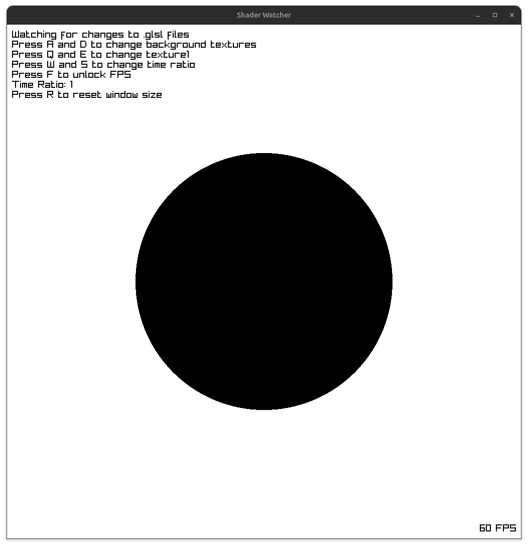
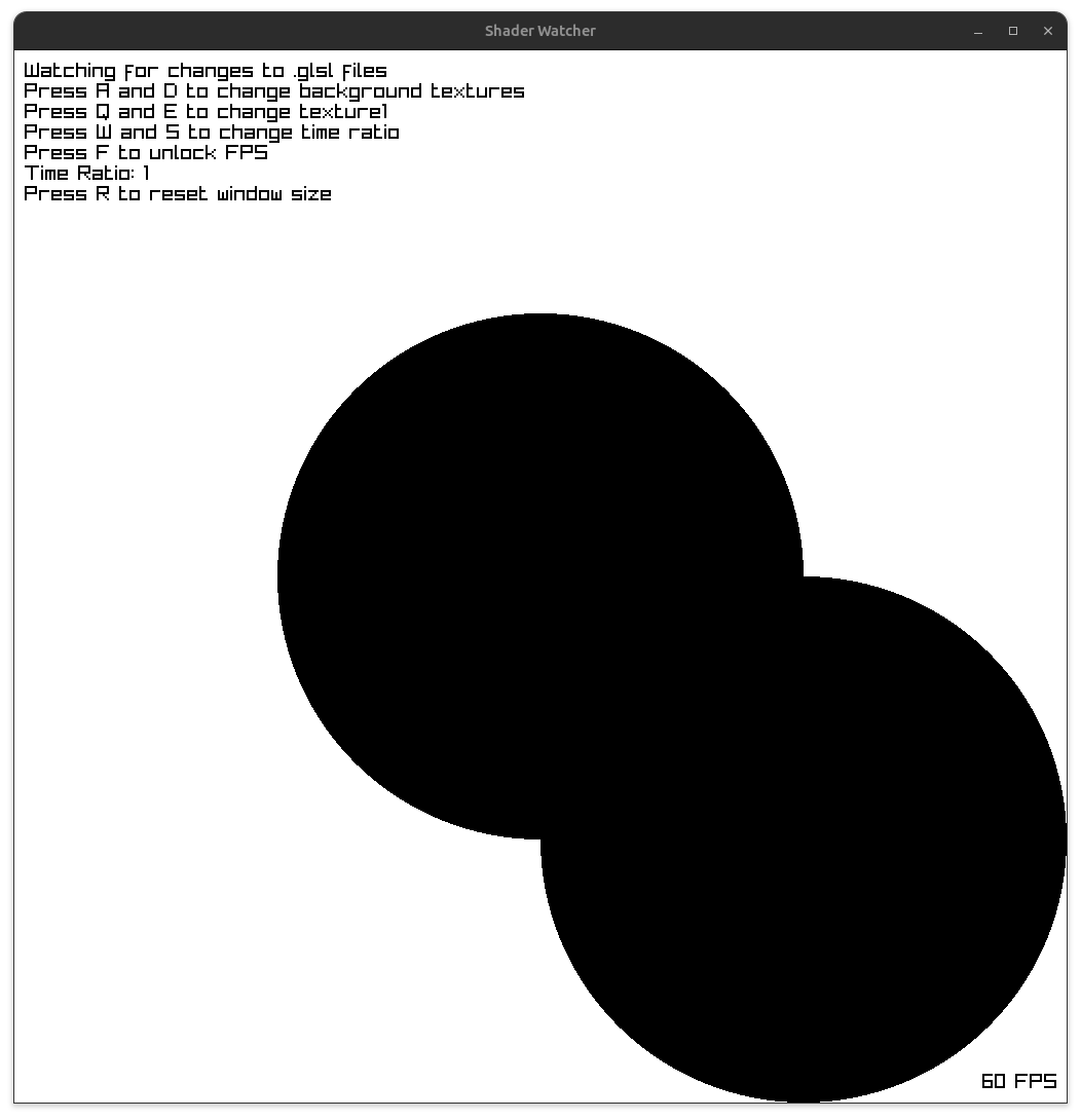
Combining Shapes

Finally, as an example of how to use this to construct some shapes, let’s combine two circles. Keeping the original circle, but adding another one at the right bottom quadrant of the screen.

void main() {
    // center the coordinate system (also the center of the first circle)
    vec2 uv = -fragTexCoord.xy * 2.0 + 1.0;
    // the center of the second circle, offset
    vec2 st = vec2(-0.5, -0.5) - uv;
    float d = sdf(uv, 0.5); // circle 1 SDF
    float e = sdf(st, 0.5); // circle 2 SDF
    float x = step(0.0, min(d, e));
    finalColor = vec4(vec3(x), 1.0);
}

Here, we use the min function to take the lowest of the two values and use it as our final output. Remember that the values within the radii are negative, so we’ll always want to use those when we’re combining shapes.

Conclusion

While this was super basic, you can end up creating some really interesting shapes by creatively manipulating the edge limits of the smoothstep function and adding them together.

For more complex 2D SDFs, I highly recommend Inigo Quilez’s wonderful articles on his site.